Defining "Mix-Shift" Analysis
Labeled “mix-shift,” “price-volume,” or “mix-rate” analysis, one of the most common analytical patterns in business is controlling for mix changes.
When a metric moves, the question is rarely just:
“Did it go up or down?”
It’s:
“Was that change driven by segment mix shifting — or by behavior changing within segments?”
This pattern shows up everywhere:
- Growth metrics like conversion or retention rates
- Price-volume analysis in logistics
- Margin % calculations in regional expansion
- ARPU and frequency metrics in subscription businesses
Yet despite how common it is, mix-shift analysis is still largely manual.
The Core Question Behind Mix-Shift
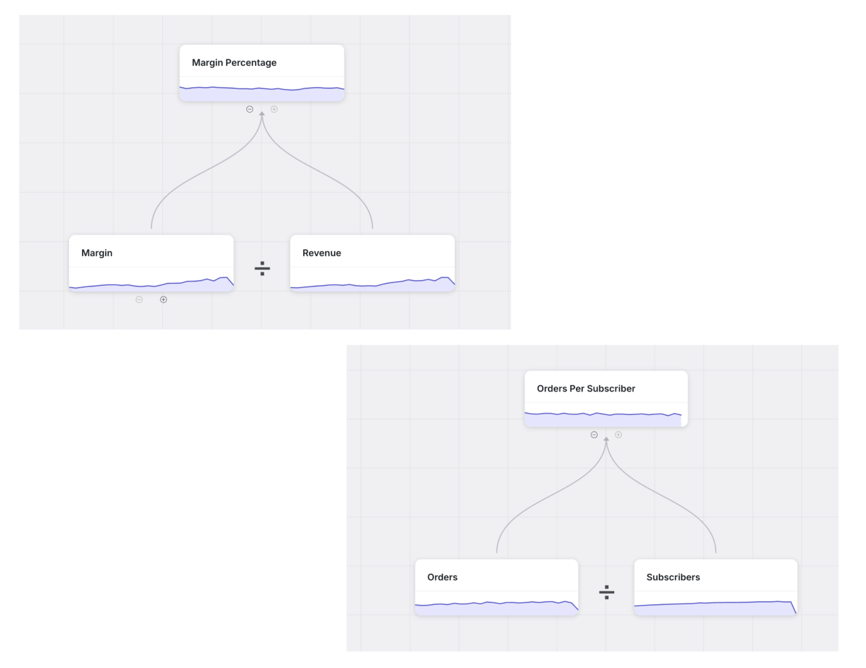
Every ratio-based metric has two fundamental components:
- Composition (size / mix)
- Behavior (rate / performance)
When a blended metric changes, the movement can be driven by:
- A change in segment sizes (mix effect)
- A change in segment-level behavior (rate effect)
- Or both
Disentangling those effects is essential for strategic clarity.
But today, it typically requires exporting data, building custom spreadsheets, and carefully constructing decomposition logic each time.
That’s friction.
Example 1: Logistics Expansion and Margin Decline
Consider a logistics provider expanding into new regions with structurally lower margin profiles.
Over several months, overall margin % declines meaningfully.
The question:
Is this decline a result of underperformance — or simply the natural consequence of expansion into lower-margin markets?
A mix-shift analysis separates:
- Size impact: How much of the change is due to shifts in regional volume?
- Behavior impact: How much is due to margin % changes within each region?
In the decomposition table:
- The Size column captures the effect of changing segment weights.
- The Behavior column captures changes in segment-level performance.
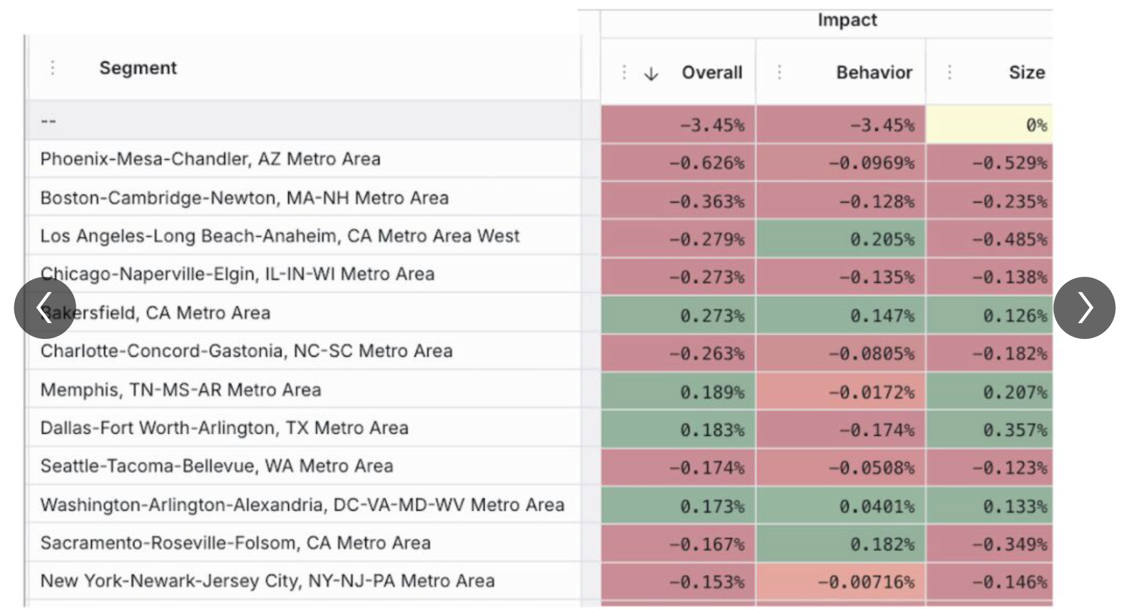
From inspecting the size contributions, you can estimate how much the contribution growth from the newer, lower margin markets like Dallas and Memphis are unable to offset the negative declines (also attributable to size) from their higher margin markets like LA and Phoenix.
Without this breakdown, leaders might misinterpret expansion strategy as operational underperformance.
With it, the conversation changes.
Example 2: Subscription Frequency and User Mix
Now consider a subscription business tracking ordering frequency.
Overall frequency declines.
Is it because customers are ordering less frequently — or because the mix of customers changed?
The decomposition again separates:
- Mix effect: Shifts in the % of users by tenure cohort
- Behavior effect: Changes in frequency within each cohort
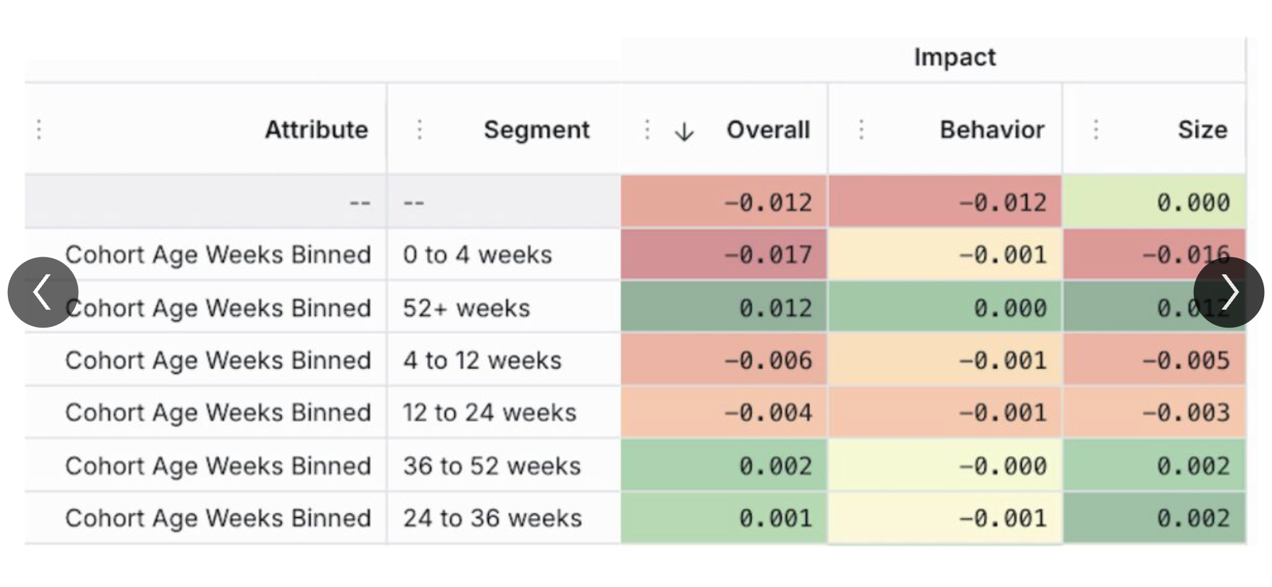
The table reveals a clear story:
The percentage of newer users (0–4 and 4–12 weeks) declines.
Older cohorts (52+ weeks) represent a larger share of the base — but they order less frequently.
Even if behavior within cohorts is stable, a shift in mix alone can drive overall decline.
This is not a tactical issue.
It’s a lifecycle composition issue.
And that distinction matters enormously for growth strategy.
Why This Analysis Shouldn’t Be Manual
Mix-shift analysis is not exotic.
It’s a structural property of ratio-based metric trees.
When metrics are modeled explicitly — especially as numerator/denominator trees — software can detect when mix decomposition is feasible and execute it automatically.
For example:
Conversion Rate = Orders / Sessions
Margin % = Profit / Revenue
ARPU = Revenue / Active Users
Frequency = Orders / Users
These structures naturally support separation into:
- Volume effects
- Rate effects
- Mix effects
When the metric tree encodes segment hierarchies and ratio relationships, algorithms can systematically attribute impact.
No custom spreadsheet required.
From One-Off Analysis to Out-of-the-Box Automation
At Trace, mix-shift analysis is one of several analyses available out of the box.
Because once the metric tree is defined:
- the numerator and denominator are explicit
- segment hierarchies are known
- dependencies are encoded
The heavy lift shifts from the human to the system.
Instead of spending four hours constructing decomposition tables, analysts receive structured attribution instantly.
And that changes the economics of analysis.
If you save four hours per analysis:
- How many more hypotheses can you test?
- How many more experiments can you evaluate?
- How much faster can leadership align?
Automation doesn’t just save time.
It increases analytical surface area.
The Broader Point
Mix-shift analysis is just one example of what becomes possible when the business is modeled explicitly.
When metric trees encode how outcomes decompose:
- decomposition becomes systematic
- attribution becomes repeatable
- automation becomes realistic
This is the difference between dashboards and analytics infrastructure.
Dashboards show metrics.
Metric trees enable reasoning.
And when reasoning can be automated, clarity scales.